OpenAI Gym and Q-Learning

Download the jupyter notebook and run this blog post yourself!

In this post, we will be making use of the OpenAI Gym API to do reinforcement learning. OpenAI has been a leader in developing state of the art techniques in reinforcement learning, and have also spurred a significant amount of research themselves with the release of OpenAI Gym.

In the previous post, we implemented Markov decision processes (MDPs) by hand, and showed how to implement $Q$-learning to create a greedy policy that significantly outperforms a random policy. The purpose of that post was to drive home the nitty gritty details of the mathematics of MDPs and policies.

However, in reality, the environments that our agents live in are not described with an explicit transition matrix $\mathcal{P}$. The MDP model is just used as a convenient description for environments where state transitions satisfy the Markov property. MDPs are useful because we can use them to prove that certain policy learning algorithms converge to optimal policies.

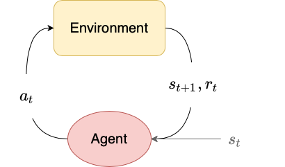
In the general reinforcement learning paradigm, the agent only has access to the state $s_t$, the corresponding reward $r_t$, and the ability to choose an action $a_t$. It does not have access to the underlying state dynamics $\mathcal{P}$ (usually because environments aren’t actually implemented using a state transition matrix).

import gym
import numpy as np; np.random.seed(0)

To use OpenAI Gym, you load an environment from a string. A list of environments is available here.

env = gym.make('FrozenLake-v0')

Gym is made to work natively with numpy arrays and basic python types. Each env (environment) comes with an action_space that represents $\mathcal{A}$ from our MDPs.

env.action_space

Discrete(4)

There are many kinds action spaces available and you can even define your own, but the two basic ones are Discrete and Box.

Discrete is exactly as you’d expect: there are a fixed number of actions you can take, and they are enumerated. In the case of the FrozenLake-v0 environment, there are 4 actions that you can take.

Box means that the actions that it expects as inputs can be floating-point tensors, which means np.ndarray of arbitrary dimension. Usually this is just a vector, for example representing torques applied to various joints in a simulated robot.

Each environment also comes with an observation_space that represents $\mathcal{S}$ from our MDPs.

env.observation_space

Discrete(16)

Like action spaces, there are Discrete and Box observation spaces.

Discrete is exactly as you’d expect: there are a fixed number of states that you can be in, enumrated. In the case of the FrozenLake-v0 environment, there are 16 states you can be in.

Box means that the observations are floating-point tensors. A common example is when the observations are images, which are represented by 3D tensors.

To interact with the environment, two steps are required.

The first step is to get the initial observation for the environment $s_0$. No action needs to be taken; the initial state is simply drawn from the distribution over initial states $s_0 \sim p(s_0)$. This is done using env.reset().

s_0 = env.reset()
s_0

0

Since the observation space is Discrete, an initial observation of 0 makes sense, since states are just enumerated.

Essentially all environments provided through Gym are episodic, meaning that eventually any trajectory will end. This can happen for a few reasons:

1. The pre-determined maximum number of timesteps $T$ has been reached.
2. The agent has reached some “goal” state or accomplished the task described by the MDP.
3. The agent has reached some “dead” state or failed the task described by the MDP.

We can actually consider all MDPs to be continuing (rather than episodic). We have some “terminal state” $s_T$ where the agent ends up, and any action simply returns them to the same state $s_T$ and provides a reward of $0$. This view of MDPs preserves the way that the return $R_t$ and discounted return $G_t$ are calculated. If we view all MDPs as continuing, then the cases above can all be considered “terminal” states.

The OpenAI Gym interface uses this definition of MDPs. When an agent is in a state $s_t$ and selects an action $a_t$, the environment provides the reward $r_t$ and next state $s_{t+1}$, as well as a done flag $d_t$. If we treat $d_t=1$ to mean “the state $s_{t+1}$ is a terminal state”, then we can modify the $Q$-learning algorithm as follows:

\[Q(s_t, a_t) \gets (1-\alpha)Q(s_t, a_t) + \alpha \left( r_t + (1-d_t) \gamma \max_{a_{t+1}} Q(s_{t+1}, a_{t+1}) \right)\]

Adding the $(1 - d_t)$ term implies that the discounted return $G_t$ is just going to be $r_t$, since all rewards after that are going to be 0. In some situations this can help accelerate learning.

When the agent reaches a terminal state, the environment needs to be reset to bring the agent back to some initial state $s_0$.

As alluded to above, the second step to interacting with the environment is to select actions $a_t$ to produce rewards $r_t$ and next states $s_{t+1}$ and terminal flags $d_t$. To do this, we use the env.step method.

a_t = env.action_space.sample()
s_t_next, r_t, d_t, info = env.step(a_t)

It also returns info which supplies information that might not be readily available through the other three return parameters. It is usually ignored.

s_t_next

0

r_t

0.0

d_t

False

info

{'prob': 0.3333333333333333}

Here’s an example of a basic loop for using Gym:

env = gym.make('FrozenLake-v0')
s_t = env.reset()
for t in range(1000):
    # no policy defined, just randomly sample actions
    a_t = env.action_space.sample()
    s_t, r_t, d_t, _ = env.step(a_t)
    if d_t:
        s_t = env.reset()

We can visualize what’s happening in the environment by calling the env.render method. For this environment, the output is a text representation of the FrozenLake maze, but for more complex environments usually a rendering of the environment will be displayed.

env.render()

env.step(env.action_space.sample())
env.render()

The FrozenLake-v0 environment has both a small discrete action space and small discrete state-space. Let’s use our $Q$-learning algorithm from the previous post to learn an optimal policy.

We are also going to add an extra bit to our algorithm by following an $\epsilon$-greedy policy. We use a parameter $\epsilon$ that determines the probability of choosing a random action versus choosing an action following the greedy policy. This can help with exploration. since at the very beginning our estimates for $Q$ are likely very wrong.

This is a good time to talk about the difference between on-policy algorithms and off-policy algorithms.

On-policy algorithms require that the data used to train the policy must be generated by the policy itself.

Off-policy algorithms can use data generated by any policy.

$Q$-learning is an off-policy algorithm. Any transition $s_t, a_t, r_t, s_{t+1}$ can be used to train the policy (i.e., to learn $Q$). Data could be collected by a random policy for all we care.

The only reason that we often use the policy itself to collect data for $Q$-learning is that by following a good policy, we can get into states that might be hard to reach using a bad (random) policy.

We implement a $Q$ learner class below that relies on the OpenAI Gym interface.

class QLearner:
    def __init__(self, env, epsilon, alpha, gamma):
        self.N = env.observation_space.n
        self.M = env.action_space.n
        self.Q = np.zeros((self.N, self.M))
        self.epsilon = epsilon
        self.alpha = alpha
        self.gamma = gamma

    def act(self, s_t):
        if np.random.rand() < self.epsilon:
            return np.random.choice(self.M)
        else:
            return np.argmax(self.Q[s_t])

    def learn(self, s_t, a_t, r_t, s_t_next, d_t):
        a_t_next = np.argmax(self.Q[s_t_next])
        Q_target = r_t + self.gamma*(1-d_t)*self.Q[s_t_next, a_t_next]
        self.Q[s_t, a_t] = (1-self.alpha)*self.Q[s_t, a_t] + self.alpha*(Q_target)

If anything in the QLearner class seems unfamiliar, revisit the previous post.

Let’s run a small training loop using an instance of QLearner.

def train(env, ql, T=1000000):
    '''
    env (gym.Env): environment
    T (int): number of learning steps
    '''
    s_t = env.reset()
    for t in range(T):
        a_t = ql.act(s_t)
        s_t_next, r_t, d_t, _ = env.step(a_t)
        ql.learn(s_t, a_t, r_t, s_t_next, d_t)
        s_t = s_t_next
        if d_t:
            s_t = env.reset()
    return ql

env = gym.make('FrozenLake-v0')
env.seed(0)
ql = QLearner(env, epsilon=0.2, gamma=0.99, alpha=0.1)
ql = train(env, ql)

We can run a similar loop to test out the performance of the algorithm. We switch to a purely greedy policy during testing.

def test(env, policy, T=10000):
    '''
    env (gym.Env): environment
    policy (callable): the policy to use
    T (int): number of learning steps
    '''
    policy.epsilon = 0
    scores = []
    s_t = env.reset()
    for t in range(T):
        a_t = policy.act(s_t)
        s_t, r_t, d_t, _ = env.step(a_t)
        if d_t:
            scores.append(r_t)
            env.reset()
    return sum(scores)/len(scores)

test(env, ql)

0.7889908256880734

Let’s compare this to a random policy:

class RandomPolicy:
    def __init__(self, env):
        self.N = env.action_space.n

    def act(self, s_t):
        return np.random.choice(self.N)

rp = RandomPolicy(env)
test(env, rp)

0.01753048780487805

We can see that the $Q$-learning algorithm significantly outperforms the random policy.

We can also take a look into what the agent has learned:

ql.Q

array([[0.57617712, 0.55583545, 0.54581116, 0.54775153],
       [0.2990091 , 0.37494937, 0.27208237, 0.52605537],
       [0.45183278, 0.43186818, 0.42052267, 0.46940612],
       [0.30306281, 0.32566571, 0.28188562, 0.4418104 ],
       [0.60072092, 0.33393605, 0.43804114, 0.33343835],
       [0.        , 0.        , 0.        , 0.        ],
       [0.3182098 , 0.12357659, 0.37948305, 0.11759624],
       [0.        , 0.        , 0.        , 0.        ],
       [0.44422165, 0.44398877, 0.58197738, 0.64138795],
       [0.56747524, 0.68729516, 0.42164102, 0.5584325 ],
       [0.65534316, 0.3897545 , 0.35962185, 0.39538081],
       [0.        , 0.        , 0.        , 0.        ],
       [0.        , 0.        , 0.        , 0.        ],
       [0.3849224 , 0.68670132, 0.72970373, 0.46354652],
       [0.76026213, 0.88506535, 0.82057152, 0.79343588],
       [0.        , 0.        , 0.        , 0.        ]])

Some rows are 0 because those rows correspond to states that are terminal and provide no reward. There are “holes” in the maze that the agent can fall through, terminating the environment.

We can use env.unwrapped to get under the hood of an env, though the attributes of the unwrapped environment are not in any way standardized and should only be used for getting a better understanding, and never for learning.

Let’s look at row 13 from the $Q$ table:

ql.Q[13]

array([0.3849224 , 0.68670132, 0.72970373, 0.46354652])

It looks like choosing action 0 is considered poor. Why might that be? Let’s force the environment into state 13 and see where that is.

env.unwrapped.s = 13
env.render()

Action 0 corresponds to going left. In this case, we would move into a hole (H). The only reason that the predicted $Q$ valued for $Q(15, 0)$ is not 0 is that the environment is ‘slippery’: sometimes when you choose an action, you move as if you had chosen a different action.

You can download the notebook here.